Interpreting Results

After running rule_significance_test(), Jesse returns a result dictionary with everything you need to evaluate whether your trading rule has genuine predictive power. Understanding how to read these results correctly is what separates a confident trading decision from wishful thinking.

The p-value

The p-value answers one question:

"If this entry rule had no next-bar edge, what fraction of bootstrap simulations would have produced a mean return as good as or better than the one I observed?"

Technically: it is the fraction of simulated means — drawn under H₀, the null hypothesis that the rule has no predictive power — that were greater than or equal to the observed mean.

p-value	Interpretation
p ≤ 0.001	Highly significant — exceptionally unlikely to be due to chance
p ≤ 0.01	Very significant — very unlikely to be due to chance
p ≤ 0.05	Statistically significant — unlikely to be due to chance
p ≤ 0.10	Possibly significant — weak evidence; treat with caution
p > 0.10	Not significant — fail to reject H₀

The lower the p-value, the less likely your rule's historical performance is the result of pure chance. A p-value of 0.02 means only 2% of random simulations matched or beat your rule's observed mean — that is strong evidence the rule captures real signal.

WARNING

A statistically significant p-value does not guarantee future profits. It only tells you that the rule's historical entry timing was unlikely to be pure chance. Real-world performance also depends on exits, position sizing, fees, slippage, and whether the market conditions that drove the signal persist into the future. Treat the result as one piece of evidence, not a green light to go live.

The observed mean

The observed mean is the average next-bar log return produced by your rule. At each bar the strategy's should_long() / should_short() methods are called to record a signal (+1, -1, or 0). The signal emitted at bar t is multiplied by bar t+1's detrended log return (the raw log return minus the overall mean log return for the period, which removes market drift). The observed mean is the average of all those products.

• A positive observed mean means the entry signals had a positive average next-bar detrended return. It does not mean the full strategy was profitable.
• A negative observed mean means the rule was systematically on the wrong side of price moves.
• A value near zero indicates little to no directional edge.

TIP

Neutral bars — where the strategy returned 0 from both should_long() and should_short() — contribute zero and remain in n_observations. Because they remain in the denominator, frequent neutral signals reduce the magnitude of the observed mean.

The annualized return

The annualized return in the result dict is a rough scaling of the bar-level observed mean:

annualized_return = observed_mean × (365 × 24 × 60 ÷ timeframe_minutes)

Jesse converts the selected route timeframe to minutes and scales the per-bar mean by the number of those bars in a 365-day crypto year. For example, a 4h route uses 6 × 365 = 2,190 bars per year, while a 1D route uses 365.

TIP

Treat this figure as a directional signal, not a precise P&L forecast. It is computed from raw bar-level log returns and ignores fees, leverage, compounding, and position sizing. A number that looks like +35% annualized here may produce very different live results once those factors are applied — in either direction.

The chart

Calling plot_significance_test(result) saves a PNG histogram to your charts/ folder. Here is what each visual element means:

• Blue histogram bars — the distribution of simulated means under H₀. This shows what the rule's performance would look like if the entry signal had absolutely no predictive power and results were purely due to chance. The bell-shaped curve centred near zero represents the full range of outcomes a random rule could have produced by luck alone.
• Red / tomato-shaded bars — the portion of the simulated distribution that equals or exceeds the observed mean. This shaded area is the p-value visualised: a larger red region means a higher (less significant) p-value; a tiny red sliver at the far right means a very low, significant p-value.
• Dashed vertical line — the observed mean from your actual strategy signals. This marks where your rule's real performance lands on the null distribution.

The further to the right the dashed line sits relative to the bulk of the blue histogram, the more significant the result. You want the dashed line deep in the right tail, with little to no red area to its right.

An info box in the top-left corner of the chart summarises the key numbers at a glance: the p-value and its significance label (★★ for very significant, etc.), the annualised return estimate, and the number of observations and simulations used.

Example chart — a very significant result

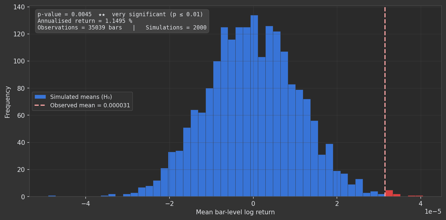
This chart is a strong example of what a genuine signal looks like visually:

• The blue histogram forms a near-perfect bell curve tightly clustered around zero — exactly what you expect from random chance. Most simulated runs produced a mean bar-level log return somewhere between −4×10⁻⁵ and +3×10⁻⁵.
• The dashed red line is pinned far into the right tail at an observed mean of 0.000031. It sits well outside the bulk of the simulated distribution — the rule's actual performance is exceptional relative to what chance alone would produce.
• The tiny red sliver to the right of the dashed line represents the fraction of simulations that equalled or beat the observed mean. Here that fraction is just 0.0045 (0.45%) — only 9 out of 2,000 bootstrap draws matched the real rule's performance, giving a p-value of 0.0045, rated ★★ very significant (p ≤ 0.01).
• The info box in the top-left confirms: p-value = 0.0045, Annualised return = 1.1495 %, Observations = 35,039 bars, Simulations = 2000.

The low annualised return estimate (~1.1%) may look modest, but remember this is a bar-level signal-only metric stripped of leverage and compounding — it indicates the entry signal itself is reliable and worth building a full strategy around.

What a non-significant chart looks like

By contrast, when a rule has no edge, the dashed line falls near the centre of the blue histogram. The red shaded region covers a large proportion of the distribution — often 50–80% or more — meaning most random simulations performed just as well or better. There is no visual separation between the rule's observed mean and what pure chance would produce.

n_observations

The n_observations field reports how many bars were actually used in the test, after the warmup period is consumed and any bars with invalid price data are removed.

More observations produce a more reliable and stable p-value:

• Fewer than 30 bars — Jesse will emit a warning. The test result is numerically unstable and should not be trusted.
• 30–200 bars — marginal; treat results with extra caution.
• Several hundred or more — the p-value is reasonably stable and the test is meaningful.

WARNING

If n_observations is very low, consider running the test over a longer date range or switching to a finer timeframe so that more bars are available for evaluation.

About the Bootstrap method

rule_significance_test() uses a stationary bootstrap that builds a null distribution by resampling random-length contiguous blocks from the rule's zero-centred return series. See the How it works page for the statistical mechanics.

What to do with the results

Significant result (p ≤ 0.05)

Your rule's entry logic shows genuine historical signal. The natural next step is a full backtest with:

• Realistic position sizing and leverage
• Fee and slippage modelling
• Drawdown analysis (max drawdown, Calmar ratio)
• Monte Carlo analysis — both candles-based and trade-order shuffling — for robustness testing

Treat the result as evidence about next-bar entry timing, then evaluate the full strategy separately. A pass is useful evidence, but it is not an entry ticket or a substitute for a backtest.

Not significant result (p > 0.10)

Fail to reject H₀. The test did not establish a next-bar entry edge. A p-value between 0.05 and 0.10 is weak evidence; above 0.10 there is no meaningful evidence for this narrow claim. This does not invalidate multi-bar holding behavior, stops, targets, sizing, or the full strategy.

WARNING

If the strategy already has exits, a failing p-value is not a reason to discard it. Entries with no edge at any horizon can still be profitable once asymmetric targets and stops are applied — see Why a profitable strategy can fail this test.

If you are screening a raw entry idea and it fails, these questions are the useful next step:

• Is the signal indicator actually predictive, or might the result be a coincidence specific to this data window?
• Have you tested over a long enough period and across different market regimes?
• Can you reformulate the entry condition to capture the underlying idea more cleanly?

Use it alongside Monte Carlo analysis

The significance test and Monte Carlo analysis are complementary tools, not competing ones:

Tool	What it validates
Rule Significance Test	Entry signal edge (signal × next-bar detrended return)
Monte Carlo — Trade Shuffling	Trade timing robustness across shuffled trade sequences
Monte Carlo — Candles-Based	Structural robustness across modified market conditions

A comprehensive validation workflow runs all three. A strategy that passes all of them has been stress-tested from multiple independent angles, giving you much greater confidence before committing real capital.

Complete worked example

Below is a print_results() helper you can add to your own research scripts, followed by example terminal output for both a significant and a non-significant case.

def print_results(result: dict) -> None:
    """Pretty-print the significance test result."""
    p = result["p_value"]
    if p <= 0.001:
        significance = "HIGHLY SIGNIFICANT (p ≤ 0.001)"
    elif p <= 0.01:
        significance = "VERY SIGNIFICANT (p ≤ 0.01)"
    elif p <= 0.05:
        significance = "STATISTICALLY SIGNIFICANT (p ≤ 0.05)"
    elif p <= 0.10:
        significance = "POSSIBLY SIGNIFICANT (p ≤ 0.10) ~"
    else:
        significance = "not significant (p > 0.10)"

    print(f"\n{'='*60}")
    print(f"  Rule Significance Test — Bootstrap")
    print(f"{'='*60}")
    print(f"  Observations      : {result['n_observations']} bars")
    print(f"  Simulations       : {result['n_simulations']}")
    print(f"  Observed mean     : {result['observed_mean']:.8f}")
    print(f"  Annualised return : {result['annualized_return'] * 100:.4f} %")
    print(f"  p-value           : {p:.4f}   →  {significance}")
    print(f"{'='*60}\n")

Example output — significant result (4h route):

============================================================
  Rule Significance Test — Bootstrap
============================================================
  Observations      : 2190 bars
  Simulations       : 1000
  Observed mean     : 0.00024041
  Annualised return : 52.6498 %
  p-value           : 0.0180   →  STATISTICALLY SIGNIFICANT (p ≤ 0.05)
============================================================

Here a p-value of 0.018 means only 1.8% of all bootstrap simulations matched or beat the observed mean under H₀. The dashed line on the chart would sit well into the right tail of the blue histogram, with a very small tomato-shaded region to its right.

Example output — not significant result (4h route):

============================================================
  Rule Significance Test — Bootstrap
============================================================
  Observations      : 2190 bars
  Simulations       : 1000
  Observed mean     : -0.00019395
  Annualised return : -42.4750 %
  p-value           : 0.7990   →  not significant (p > 0.10)
============================================================

Here 79.9% of bootstrap simulations performed equally well or better. There is no meaningful evidence of genuine signal — the dashed line on the chart would sit near the centre of the blue histogram, with a large red region to its right.

Caveats and limitations

Keep the following in mind when interpreting any result from rule_significance_test():

• Fixed horizon by construction — the test measures direction over the single bar that follows each signal. Edges that come from asymmetric targets and stops, variable holding periods, or position sizing are invisible to it, which is why a profitable strategy can fail this test.
• Entry signal only — the test runs a signal-only simulation. It records when your strategy's should_long() / should_short() methods fire, but no orders are ever submitted. Exits, stop-losses, take-profits, position sizing, and fees are completely absent from the calculation.
• A weak signal is not a dead end — a borderline or even insignificant signal can still be made profitable with smart position sizing, tight risk management, and well-timed exits. Conversely, a highly significant signal can be eroded to nothing by poor exit logic or high fees.
• Minimum observations matter — the test is most reliable with at least several hundred bars. Fewer than 30 observations produces a numerically unstable p-value; a few dozen data points are simply not enough to reliably distinguish signal from noise.
• In-sample only — the test is run on the same historical data you supply. Statistical significance on in-sample data does not imply out-of-sample significance. Always validate on a held-out period or via walk-forward analysis before trading live.
• Single route enforced — rule_significance_test() accepts exactly one trading route. For multi-symbol or portfolio-level analysis, run the function separately for each symbol and compare the individual results.